Wrap texture adressing within a sprite sheet or atlas

FEZ shipped with volume textures (aka 3D textures) for all the sprite animations in the game. Gomez, NPCs and other animated pixel art were all done using those. This was a tech call that I made way back in 2008 and kept with it because it makes more sense than you might think :

  • No need to do texture packing and keeping track of where frames are in the sheet; a volume texture is an ordered list of 3D textures, every frame is a slice!
  • The pixel shader just does a tex3D() call with the Z component of the texture coordinates being the step of the animation between 0 and 1.
  • Cool side-effect : hardware linear interpolation between animation frames! This wasn’t very useful for me (except for one thing, water caustic overlays), but it’s a nice bonus.
  • Mip-mapping with 3D textures is problematic because it downsizes in X, Y and Z, meaning that each mip level halves the number of frames. However, I didn’t need mip mapping at all (for sprites), I never undersample pixel art.
  • Same limitation when making a volume texture power-of-two, it also goes power-of-two in the Z axis which means a lot of blank frames, which is wasteful but not a huge problem to deal with.

But while I haven’t done real testing, one can assume that they’re slower than a regular 2D sprite sheet, and they imply that you have one texture by animation, which restricts how much you can pack things together. Creating a volume texture at load-time with XNA Texture2D.SetData() calls means one call per animation frame, which is noticeably slow. Also, volume textures are not currently supported by MonoGame, and I assume some integrated graphics hardware would have trouble dealing with them.

So the more traditional alternative is using a sprite sheet, which is easy to make using tools like the Sprite Sheet Packer.

But then what if you need to use wrap texture addressing on it, to have horizontally and/or vertically repeating textures?

If you only repeat on one axis, have relatively small textures and a small number of frames, you can force the texture packer to layout the sprites on a single row or column, which allows wrapping on the other axis.

This worked for some animations, but some were just too big or had too many frames to fit it in under 4096 pixels. In that case, there’s one final option : pixel shaders to the rescue!

When addressing the texture in your shader, you’re likely to use a 3×3 texture matrix, or a 4D vector if you’re short on input parameters. Either way, you have four components : UV offset and UV scale. You can use those to manually wrap the texture coordinates on a per-pixel basis. In the sample below, I extract the data from a texture matrix.

Vertex Shader

Out.TextureCoordinates = mul(float3(In.TextureCoordinates, 1), Matrices_Texture).xy;
Out.UVMinimum = Matrices_Texture[2].xy;
Out.UVScale = float2(Matrices_Texture[0][0], Matrices_Texture[1][1]);

Pixel Shader

float2 tc = In.TextureCoordinates;
tc = frac((tc - In.UVMinimum) / In.UVScale) * In.UVScale + In.UVMinimum;
float4 sample = tex2D(AnimatedSampler, tc);

The frac() HLSL intrinsic retains the decimal part of its input, which gives the normalized portion of the texture that the coordinates are supposed to show. Then I remap that to the sprite’s area in the atlas, and sample using those.

I ended up only needing wrapping on one axis for that big texture/animation, but this code does both just in case. This is WAY simpler than customizing the vertex texture coordinates to allow wrapping.
One caveat though, this won’t play well with linear filtering. Since FEZ is pixel art, I could get away with point sampling and had no artifacts there.

P.S. A simple fix to enable usage of linear filtering : pad the sprites with 1 pixel column and rows of the opposite side of the texture! (and don’t include those in the sampled area; it only gets sampled by the interpolator)
Cubes All The Way Down @ MIGS

Back in November 2011, I gave a talk at the Montréal International Game Summit in the Technology track called “Cubes All The Way Down”, where I talked about how FEZ was built, what’s the big modules, the challenges and intricacies of making a tech-heavy indie game from scratch.

It went okay.
I was really stressed, a bit unprepared due to FEZ crunch time, and just generally uncomfortable speaking in front of an audience.
I spoke so fast that I finished 15 minutes early and had 30 minutes for questions, which worked great for me because the relaxed setting of a Q&A session meant better flow, better information delivery, I really liked that part. Also I had friends in the front row that kept asking good questions and were generally supportive, so all in all a good experience. :)

I was asked about giving the slides out, so here they are! Unedited.

It’s Cubes All The Way Down (Powerpoint 2007 PPTX format) (PDF format)

Enjoy!

Encoding boolean flags into a float in HLSL

(this applies to Shader Model 3 and lower)

Hey! I’m still alive!

So, imagine you’re writing a shader instancing shader (sounds redundant, but that’s actually what they are) and you’re trying to pack a lot of data into a float4 or a float4x4 in order to maximize the amount of instances you can render in a single draw call.

My instances had many boolean flags that changed per-instance and that defined how they were lit or rendered. Things like whether or not they are fullbright (100% emissive), texture transform flags (repeating on x or y, more efficient to rebuild the texture matrix than pass it), etc.
Using one float out of your instance data matrix for each boolean is doable, but highly wasteful. A natural way to fit in many flags into an integer is to use a bitfield, but there’s no integer arithmetic in HLSL, and they’re floating point values… how does one proceed?

Here’s how I did it.

Application side

First, this is how I pack my data into floats from the application side (setting the effect parameter) :

int flags = (fullbright ? 1 : 0) | 
	(clampTexture ? 2 : 0) | 
	(xTextureRepeat ? 4 : 0) | 
	(yTextureRepeat ? 8 : 0);

Geometry.Instances[InstanceIndex] = new Matrix(
	p.X, Rotation.X, Scale.X, color.X,
	p.Y, Rotation.Y, Scale.Y, color.Y,
	p.Z, Rotation.Z, Scale.Z, color.Z,
	Animated ? Timing.Step : 0, Rotation.W, flags, Opacity);

Just putting an OR operator between the flags you wanna put, and keep the flag bits powers of two.
Ignore the rest of the matrix contents, they’re just here for show. (in my case : position, rotation, scale, color, opacity, animation frame and the flag collection).

A note on floating point : in a single-precision floating point number as defined by the IEEE, you’ve got 23 bits for the significand. That means you can theoretically put 23 flags in there! That’s a lot of data.
(also, considering the decimal point is floating, you can effectively put much more than 23 bits if some of them are mutually exclusive…!)

Vertex shader

Now in the vertex shader, they get passed to an effect parameter through vertex shader constants, and here’s now the decoding works :

int flags = data[2][3];

bool fullbright = fmod(flags, 2) == 1;
bool clampTexture = fmod(flags, 4) >= 2;
bool xTextureRepeat = fmod(flags, 8) >= 4;
bool yTextureRepeat = fmod(flags, 16) >= 8;

I know my flags reside in the 3rd row, 4th column of my matrix, so I grab ’em from that. Might as well cast them to an integer right now since I won’t be using decimals.

Then I can test for values by testing the remainder of the division of each power-of-two. There is no integer modulo intrinsic function in HLSL for Shader Models 3 and lesser, but the floating-point version works fine.

If I set the first (least significant) bit of a number and divide it by two, the remainder will be 1 if that bit is set. Basically, we test if that number is odd or even; odd means the bit is set.

For every other test, we can test whether the remainder is greater or equal to half the divisor. Effectively, we’re masking the bits greater than the one we’re testing, and testing remaining bits for the presence of the one we’re looking for. Here, if we test for the 3rd bit (from the LSB), so masking with 8 (1000 in binary) and testing against 4 (0100 in binary) :

0000 % 1000 = 0000 // 0 < 4, bit not set
0100 % 1000 = 0100 // 4 >= 4, bit set
1011 % 1000 = 0011 // 3 < 4, bit not set
1110 % 1000 = 0110 // 6 >= 4, bit set
1101 % 1000 = 0101 // 5 >= 4, bit set

Enjoy!

Smart Screen-Space Blurring for Shadows

I’ve been working on a screen-space solution for blurring shadows that has the following features :

  • Variable-sized kernel based on surface distance and view angle
  • Rejection of samples if they lie on a non-contiguous surface, by identifying depth and normal discontinuities
  • Bilateral, two-pass blur filter to maximize the possible kernel size
  • Vertex and pixel shader 3.0, so no worry about 64 instructions in the PS

…but also works with the following constraints, to simplify matters :

  • Flat surfaces only, no curves! (to simplify the sample rejection process)
  • Full control over the rendering pipeline, so the “main render” pass can output weird values in order to be properly blurred

I quickly realized that it’s very hard or impossible to do a variable-sized Gaussian filter in real-time. If you change the kernel size, you change the standard deviation, and you need to recalculate the weights… this is too heavy for a pixel shader. So I chose to use a box filter with uniformly-spaced samples.
I totally would’ve liked to use Poisson-Disk distribution, but it’s not doable in a two-pass bilateral scenario. And you can’t achieve big kernels in real-time without separating the process in two passes.

My XNA3 implementation currently uses no additional render targets (!) but just a “resolve texture”, and resolves from the main buffer quite a lot. A R32F (Single) render target is used for the shadowmapping process itself, but otherwise everything’s done with a A8R8G8B8 (Color) main buffer.
The shadowmapping solution is standard orthographic/directional depth testing, but I’m using Exponential Shadow Maps (ESM) to simplify the depth biasing problems. I could never get my hands on a really good way to do Slope-Scale Biasing for standard depth testing, so ESM saves the day here. Otherwise, there’s no fancy cascading, splitting or projection tricks.

Here’s how it looks at different distances. The blur kernel stays approximately the same size in world-space even if the whole process is screen-space!

I’ll keep working on a clean sample to show, and I’ll definitely release the HLSL code if I can’t release the source to the whole thing. Stay tuned!

Reflective Floor

Nov. 13th Update : Added fresnel term, min/max reflection factors, pixel-perfect sampling.

Back in TV3D land for a minute!

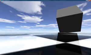
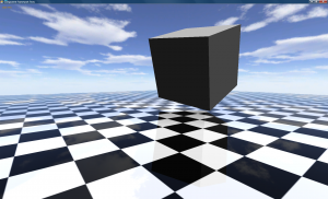
bigpic1bigpic2

(the reflection looks offset in these pics but it’s fine in realtime… not sure why it messed up here.)

Description

It might sound like an easy thing to do, but planar reflections are pretty challenging to do per-pixel. It involves a texture projection shader, some pretty scary matrix play, and so on and so forth. So I decided to make a proper sample that shows how I did it in my reflective water sample, but in its simplest expression.

The floor uses two mesh groups, one for the reflection and one for the actual floor with texture. This makes it possible to only use a shader on the reflection group, and then the other one uses standard TV3D rendering.
Sadly, it’s impossible to do per-pixel reflections without a shader. Thinking about it, an even simpler way would be to use the stencil buffer, but then if you’re working with pixels you can apply fun effects like bump-mapping and fresnel attenuation.

Update Notes

The updated version has fresnel per-pixel attenuation, which means that grazing angles will get full reflection and looking down on the floor will get next to none. The amount of reflection and the effect of the fresnel term can be tweaked with constants.
In order to make this thing work, I had to make it 3-pass :

  1. The first pass is the standard texture mapping one, without shader;
  2. The second pass multiplies the inverse of the fresnel term with the texture-mapped mesh, so that the reflection won’t be overpowering when we blend it in;
  3. The third and last pass additively-blends the reflection with fresnel applied.

The two last passes use the shader, but since both shader passes are enabled, I only need a single group for both. Nice and clean!

I also removed the texel offset thing because if you point-sample the texture (which you should, unless you’re bump-mapping), it’s pixel-perfect without any needed fix. And the blending modes and depth-write flags are moved to the shader, to make things even cleaner!

Download

Binaries + Code : PlaneReflection_src_bin.zip (8.7 Mb – C#3 VS2008 Solution)

Just the code : Projection.fx (the shader) and PlaneReflection.cs (the component that draws everything)

Enjoy!

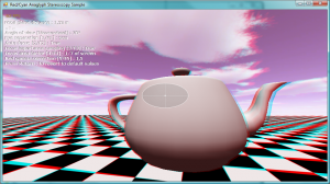
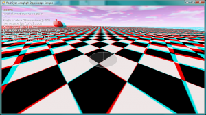
Anaglyph Stereoscopic Rendering in First Person

I decided to finally finish up my analgyph stereoscopy sample, and cut the depth-of-field component that was adding too much complexity for my limited spare time right now.

stereoscopy finalstereoscopy final 2

Download

Binaries : stereoscopy_bin.zip (1.9 Mb – Binaries)
Code : stereoscopy_src.zip (524 Kb – Source Only, get DLLs for TV3D and SlimDX from the Binaries)

Description

This sample demonstrates a couple of things :

  • Optimized anaglyph filters for red/cyan stereoscopic rendering, to reduce eye-strain by minimizing retinal revialry but still keep some color information. As my source suggests, I’ve also implemented red channel gamma correction in the shader.
  • Auto-focus of both eyes on a focal plane. The camera is in the first person and the two “virtual cameras” act like human eyes, in the manner that they are connected to a single brain that wants to look at a single point. So the center of the screen is assumed to be that focal point, and both eyes will look at it. I used a depth rendering pass to achieve this, and a weighted sum of a certain portion of the screen near the center (this is all tweakable in realtime)

The distance between the eyes is also tweakable, if you want to give yourself a headache.

I wanted to do a stereoscopy sample to show how I did it in Super HYPERCUBE, but I can’t/don’t want to release its source, so I just re-did it properly. Auto-focus is a bonus feature that I wanted to play with; sHC didn’t need that since the focal plane was always the backing wall.

This sample, like all my recent ones, uses the latest version of my components framework. There are some differences between this release and the Stencil Rendering one, but it’s mostly the same. The biggest thing is that base components (Keyboard, Sound, etc.) are not auto-loaded anymore, and must be added in the Core.Initialize() implementation. This way, if I don’t need the sound engine, I just don’t load it… makes more sense.

Hope you like it!

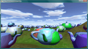
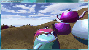
Stencil Rendering

Here’s a little demo to show off a technique that Farbs posted about earlier this week.

yay yay2

Download

Binaries : stencilrendering_bin.zip (3.6 Mb – Binaries)
Code : stencilrendering_src.zip (1.8 Mb – Source Only, get DLLs for TV3D and SlimDX from the Binaries)

Description

Every frame, a random color from the target image is sampled. This color will be used as a stencil, such that every pixel whole target color is close enough to that stencil’s color will be painted. It’s a constructive painting process; every frame paints a single color, but if you wait long enough in a single spot you’ll end up with the target image.

Actually, the post processing draw code is so concise that I can post it here :

public override void PostDraw()
{
    targetBuffer.BltFromMainBuffer();
    targetBuffer.SetSystemMemCopy(true, true); // Lolworkaround

    // 1) Pick a colour from target image
    var pickedColor = Globals.DecodeRGBA(TextureFactory.GetPixel(targetBuffer.GetTexture(), RandomHelper.Random.Next(0, targetBuffer.GetWidth()), RandomHelper.Random.Next(0, targetBuffer.GetHeight())));
    stencilShader.SetEffectParamVector3("stencilColor", new TV_3DVECTOR(pickedColor.r, pickedColor.g, pickedColor.b));
    Screen2DImmediate.Draw_FullscreenQuadWithShader(stencilShader, 0, 0, 1, 1, mainBuffer.GetTexture(), targetBuffer.GetTexture());
    mainBuffer.BltFromMainBuffer();
}

“targetBuffer” and “mainBuffer” are just two TVRenderSurfaces as big as the viewport. Since I sample from targetBuffer, it needs to be flagged with “system memory copy”. I thought this would slow things down, but it runs at very interactive framerates (60 and more).

And uh… The “lolworkaround” is a bug in the current build of TV3D. Usually you only need to set this once at initialization time, but a BltFromMainBuffer does not flag the surface as dirty and it prevents updates to the pixels that I sample. Resetting the memory copy mode makes the changes effective. Sylvain tells me it’s fixed in the current development build. :)

A pixel shader does the rest :

float4 PS(PS_INPUT IN) : COLOR 
{
	float3 bufferSample = tex2D(MainBufferSampler, IN.TexCoord).rgb;
	float3 targetSample = tex2D(TargetSampler, IN.TexCoord).rgb;

	// 2) Calc difference between current screen and target (per channel subtraction, abs, then accumulate all three into one)
	float sampleDiff = distance(bufferSample, targetSample);

	// 3) As above, but between colour picked in step 1 and target image
	float stencilDiff = distance(stencilColor, targetSample);

	// 4) Where result of step 2 > result of step 3, draw colour picked in step 1
	float4 color;
	if (stencilDiff < sampleDiff)
		color = float4(stencilColor, 1);
	else
		color = float4(bufferSample, 1);

	return color;
}

I think it’s a lovely effect. It’s very dependent on how colorful and contrasted the scene is, and it works differently for sharply-defined shapes or gradients… And of course camera movement is a big factor. In the video it gets confusing, the effect is more “painterly” if you just rotate the camera in small circles and wait for the effect to accumulate.

Isotropic Specular Reflection Models Comparison

I’ve decided to repost all my remaining TV3D 6.5 samples to this blog (until I get bored). These are not new, but they were only downloadable from the TV3D forums until now!

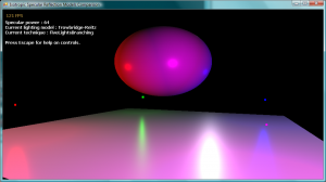
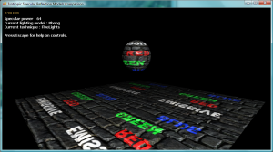
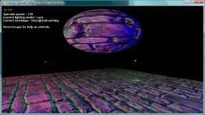
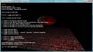
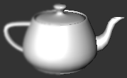
This demo (originally released as VB.Net 2005 on Feburary 13th, 2007 here) is a visual and performance comparison (and reference implementation) of five different per-pixel lighting models for isotropic specular reflections :

  • Phong reflection model
  • Blinn-Phong (Blinn D1, Phong) specular distribution
  • Lyon halfway method 1 (for k=2 and D = H* – L)
  • Trowbridge-Reitz (Blinn D3) specular distribution
  • Torrance-Sparrow (Blinn D2, Gaussian) specular distribution

My main goals were to :

  • Make an optimized HLSL implemention of each model that fits in a single Shader Model 2.0 pass and supports 3 lights
  • Evaluate the performance of each model in a multiple light, per-pixel rendering context
  • Determine which model keeps the most numerical precision and does not produce artifacts when used with normal-mapping

Download

IsotropicModels.zip [2.7 Mb] – C#3 (VS.NET 2008, TV3D 6.5 Prerelease .NET DLL Required)

Screenshots

lyon 2lyon 7
lyon 8lyon 9

Details

The HLSL shader supplied with this sample was made to mimic the built-in TV3D offset-bumpmapping shader as closely as possible. As a result, almost all of its effect parameters are mapped to standard semantics. It supports :

  • One colored directional light
  • Two colored point lights in SM2.0, and four in more recent models (SM2a/b and SM3)
  • Support for all types of vertex fog
  • Parallax mapping of texture coordinates using a grayscale heightmap
  • Diffuse mapping with alpha support (a.k.a. texturing)
  • Normal mapping
  • Specular mapping (using the alpha channel of the normalmap)
  • Emissive mapping (colored!)
  • Usage of all material terms (diffuse, ambient, specular, emissive, power and opacity)

There is no support for point light attenuation as this would’ve gone over the 64 instructions limit of the ps_2_0 profile. (also TV3D doesn’t provide semantics for these)
There is no support for spot lights for the same reasons, but I believe spots will be processed as regular point lights, ignoring the specific parameters.

Techniques

With the realtime controls, you can choose from three different techniques : FiveLightsBranching, FiveLights and ThreeLights. On SM2.0 hardware, only the third option will be valid.

The FiveLightsBranching mode uses loops and “if” statements to produce dynamic branching on SM3.0 compatible hardware. This can (but may not) be benificial because only the calculations for enabled lights are performed.
The FiveLights and ThreeLights modes respectively do five and three lights (WHAT YOU SAY !!) but all in a static manner. It does not just unroll the loop! Most of the calculations are done with matrices, which makes it more efficient on most hardware.

To keep the shader “simple” (or to prevent from becoming even more complex…) I decided not to implement a multipass 5 lights technique for SM2.0… sorry!

Blinn vs. Phong

There’s two major categories in the models I tested : the ones that use the halfway vector, and the Phong model that works with the reflected vector. (see the Wiki entry on Blinn-Phong for details on these vectors).

BlinnvsPhong
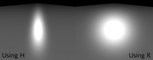
A directional light reflecting on a surface with a power value of 64

According to a paper from Siggraph 2004 called Experimental Validation of Analytical BRDF Models, the halfway methods generate specular highlights with more realistic shapes than the Phong model. I realized that myself when working on an ocean rendering shader that had a Phong specular reflection, and it was impossible to get a long grazing highlight when the sun was setting.

Normal Mapping Artifacts

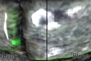
One of the things that made me do this whole analysis is that I was dissatisfied with the image quality of Phong and Blinn-Phong when used with a normal map, so per-pixel lighting. I had huge block artifacts on my water surface, and everything with a high enough specular power value and a bumpy surface. So I found about a reformulation of the Blinn-Phong model by Richard F. Lyon, written in 1993 (!) for Apple. (trivia : Mr. Lyon also invented the optical mouse… how awesome is that!)

lyonblinn

This reformulation is interesting because it does not use the specular power literally as an exponentiation, it uses a distance metric and a much lower power value to produce very similar results to the Blinn-Phong model. Using a high specular power (32 or more) hurts floating-point accuracy, even in full-precision mode.

That said, I have seen hardware that do not have this problem. I am starting to think that it may be a driver issue, or something about mobile GPUs… In any case, the safe thing to do is choose the model that never produces artifacts, right?

The Other Blinn Distributions

The two other models I implemented (Trowbridge-Reitz and Torrance-Sparrow) were “ported” from the MATLAB code in Lyon’s reformulation paper. I wanted to test them out to see if they had the same artifact problems, and how different they looked from the classic models.

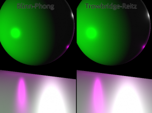
trowbridge

Trowbridge-Reitz is an interesting model because of how it looks. It’s slower than Blinn-Phong, but it has a distinct smoothness to it. The falloff of its specular highlights is softer than the other models… I’m not sure if it’s more accurate, but it looks pretty. Sadly, it has the same problems with normal mapping.

Torrance-Sparrow is a visual identity to the Blinn-Phong model. It’s the same thing, but slower and more instruction-heavy. It does not even fit in SM2.0 with 3 lights,… So I suggest you disregard it for realtime graphics.

Performance

I found that performance varies a lot depending on which technique you use, which shader model you support, how much your GPU is fillrate-limited instead of arithmetic-limited… So I’ll just say this : the Lyon model looks great, and it’s simple and fast enough to be worth considering. If you don’t experience the artifacts I describe, then the Blinn-Phong model is your best shot, but test Trowbridge-Reitz to see if it’s fast on your hardware.

It’s also worth mentioning that many things could be optimized by factorizing equations into small 1D or 2D textures (or perhaps a normalization cubemap), if your GPU loves pixels and hates instructions. But I don’t believe that the shader can be optimized that much by reorganizing code or removing useless statements. At least not without hurting visual quality.

Component System Updates

This sample contains a major breaking change to my component framework : The Service baseclass is gone. This makes Components able to “be” services (and publish many service interfaces), and allows this sample to have a much simpler class structure… no more state classes! The components just publish whatever data they want via their service interfaces. And with the new Eventful<T> class, it’s really easy to propagate changes from a controller to a view.

Gaussian Blur Revisited, part two

First part can be found here.
An implementation of the concepts presented in this series can be found here.

The Perfect Sigma

The last post’s closing note was, how are we to find the “perfect” standard deviation for a fixed number of taps such that exactly 0% of light is lost. This means that the sum of all taps is exactly equal to 1.

It’s absolutely possible, but to find this exact σ with algebra and possibly calculus was a bit over my head. So I just “binary-searched” across the decimals until my Excel grid told me that as long as double-precision goes (15 significant numbers), I have ≈ 1 as the sum. I ended up with the following numbers :

  • 17-tap : 1.2086
  • 15-tap : 1.1402108
  • 13-tap : 1.067359295
  • 11-tap : 0.9890249035
  • 9-tap : 0.90372907227
  • 7-tap : 0.809171316279
  • 5-tap : 0.7013915463849

17-taps per pass, so basically 289 effective texture samples (actually 34…), and a standard deviation of 1.2?! This is what it looks like, original on right, blurred on left :


So my first thought was, “This can’t be right.”

Good Enough

In my first demo, I used a σ = 2.7 for 9 taps, and it didn’t look that bad.
So this got me thinking, how “boxy” can the Gaussian become for it to still look believable? Or, differently put, how much light can we lose before getting a Box-like filter?

To determine that, I needed a metric, a scale. I decided to use the Mean Difference, a.k.a. Average Deviation.
A Box filter does not vary, it’s constant, so its mean difference is always 0. By calculating how low my Gaussian approximations’ mean difference goes, one can find how similar it really is to a Box filter.

The upper limit (0% box-filter-similarity) would be the mean difference of a filter that loses no light at all, and the lower limit (100% similarity) would be equal to a box filter at (again) 15 significant decimal numbers.

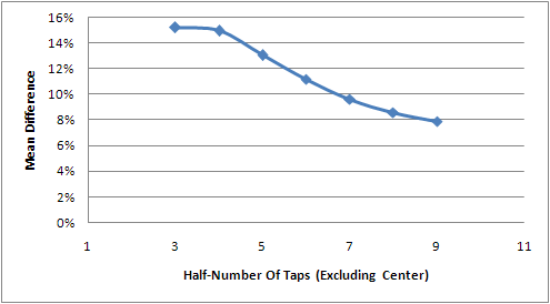
So I fired up Excel and made those calculations. It turns out that at 0% lost light, the mean difference is not linear with the number of taps. In fact, the shape highly resembles a bell curve :

I fitted this curve to a 4th order polynomial (which seemed to fit best in the graph) and at most, I got a 0.74% similarity for 0% lost light, in a 9-tap filter. I’m not looking for something perfect since this metric will be used for visual comparison; the whole process is highly subjective.

Eye Exam

Time to test an implementation and determine how much similarity is too much to this blogger’s eye.
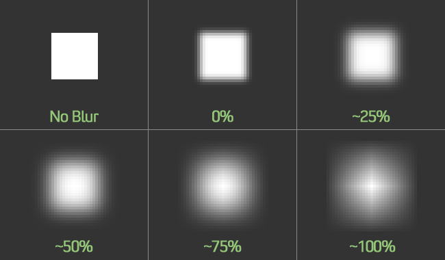
Here’s a fairly tiny 17×17 white square on a dark grey background, blurred with a 17-tap filter of varying σ and blown up 4 times with nearest-neighbour interpolation :

The percentage is my “box-likeness” or “box filter similarity” calculation described in the last section.

Up to 50%, I’m quite pleased with the results. The blurred halo feels very round and neat, with no box limit that cuts off the values harshly. But at 75%, it starts to look seriously boxy. In fact, anything bigger than 60% visibly cuts the blur off. And at 100%, it definitely doesn’t look like a Gaussian, more like a star with a boxy, diamond-shaped blur.

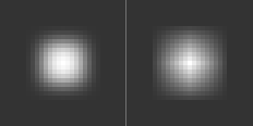
Here’s how 60% and 100% respectively look at a 9-tap, for comparison :

50% looks a liiiiiitle bit rounder, but 60% is still very acceptable and provide a nice blurring capability boost.

Conclusion

My conclusion, like my analysis, is extremely subjective…
I recommend not using more than 60% box-similarity (as calculated with my approach) to keep a good-looking Gaussian blur, and not more than 50% if your scene has very sharp contrasts/angles and you want optimal image quality.

The ideal case of 0% lost light is numerically perfect, but really unpractical in the real world. It feels like a waste of GPU cycles, and I don’t see any reason to limit ourselves to such low σ values.

Here’s a list of 50% and 60% standard deviations for all the tap counts that I consider practical for real-time shaders :

  • 17-tap : 3.66 – 4.95
  • 15-tap : 2.85 – 3.34
  • 13-tap : 2.49 – 2.95
  • 11-tap : 2.18 – 2.54
  • 9-tap : 1.8 – 2.12
  • 7-tap : 1.55 – 1.78
  • 5-tap : 1.35 – 1.54

And last but not least, the Excel document (made with 2007 but saved as 2003 format) that I used to make this article : Gaussian Blur.xls

I hope you’ll find this useful! Me, I think I’m done with the Gaussian. :D

Gaussian Blur Revisited, part one

Second part can be found here.
An implementation of the concepts presented in this series can be found here.

A long time ago, in a blog not so far away, I studied how the Gaussian distribution worked to implement a Gaussian Blur HLSL shader. That worked pretty well, I learned a lot of stuff, and managed to make a very functional shader. But some problems were overlooked and fixed with not-so-scientific solutions/hacks. Last week and this week, I spent more time thinking and experimenting with Gaussian blur weights, and discovered some pretty interesting stuff.

Losing Light

The first problem that I mention in my original post is the fact that when passing any image through a Gaussian blur shader darkens it, a certain portion of brightness or “light” is lost in the process.
Usually, the Gaussian function (a.k.a. the bell curve or normal distribution) has an integral between from x = -∞ to +∞ of exactly 1. But when you sample it at discrete intervals, you always lose a certain portion of that full integral.
To prevent this effect, I decided to “normalize” all the weights (a weight being a sample of the G(x) function at some x distance) to have a sum of exactly one, since that’s what I want to end up with anyway. This works, and my filtered images are bright again.
But doing so has a subtle yet perverse effect to it.

Boxing the Gaussian

Let’s take a 5-tap uni-dimensional kernel with a standard deviation of σ = 1. As a reminder, the standard deviation defines how wide the function is, and how much blurring is performed, and the “tap” count is the number of texture samples done in a single pass (each pass being either horizontal or vertical).
Here are the weights acquired from the function, then the normalized weights (since the function is reflective at x = 0, I only show values for [0, 2]) :

0.39894228, 0.241970725, 0.053990967
Σ = 0.990865662

0.402619947, 0.244201342, 0.054488685
Σ = 1

That looks quite fine. Now let’s use a wider σ of 5.

0.079788456, 0.078208539, 0.073654028
Σ = 0.38351359

0.208045968, 0.203926382, 0.192050634
Σ = 1

Notice how the normalized weights are very close to each other. In fact, it highly resembles an averaging 5-tap Box filter :

0.2, 0.2, 0.2
Σ = 1

When you think about it’s it very natural for this effect to occur. The bigger the standard deviation, the closer to the curve’s apex you sample values, and the lower the apex as well. So the difference between the samples is smaller and you go closer to a straight line.
In fact, at σ = ∞, any normalized Gaussian kernel becomes a Box filter. I don’t have a formal proof for that, but it’s clearly visible, and with single-precision floats it takes a lot less than the infinity.

Visual Difference

Now why is it so bad to use a box filter? It’s as wide as our kernel can get with its limited number of taps after all…

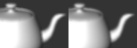
Here’s a visual comparison of the same scene under a 5-tap Box filter and a Gaussian with σ ≈ 1.5, giving it about the same span. It’s not an apples-to-apples comparison, but it should give you an idea.

Comparison shot 1

Comparison shot 2

A Box filter is quite unlike a Gaussian blur. Sharp edges get blocky and it gives a more “sharp” feel than the Gaussian. So it’s definitely not optimal.

Ye Olde Cliffhanger

Getting late here, so I’ll wrap this up.
The question left is this one : At which standard deviation does our Gaussian sampling lose 0% brightness/light for a fixed number of taps? Is that even possible?
Why, yes, yes it is. I’ll keep this for part two!