A follow-up to this article with clarifications and corrections to the “real-world considerations” can be found here.
I researched gaussian blur while trying to smooth my Variance Shadow Maps (for the Shadow Mapping sample) and made a pretty handy reference that some might like… I figure I’d post it for my first “Tips” blog post. :)
The full article contains a TV3D 6.5 sample with optimized Gaussian Blur and Downsampling shaders, and shows how to use them properly in TV3D. The article also contains an Excel reference sheet on how to calculate gaussian weights.
Update : I added a section about tap weight maximization (which gives an equal luminance to all blur modes) and optimal standard deviation calculation.
The theory
The gaussian distribution function can be expressed as a 1D function – G(x) – or a 2D function – G(x, y). Here they are :


In these functions, x and y represent the pixel offsets in relation to the center tap, in other words their distance in pixels away from the center tap. The center tap is the center from which all samples will be taken. The whole distribution can be offset by a “mean” parameter, which would displace the center tap, but that is of no use when blurring; we want the distribution to be centered.
The σ symbol is a non-capitalized greek “sigma”, which is often used in statistics to mean “standard deviation“. That’s exactly what it means here; the standard deviation of the Gaussian distribution, so how much the function is spread. The standard value is 1, but putting a greater value will spread the blurring effect on more pixels.
The e symbol in this context is Euler’s Number, ~2.7. And of course, π is Pi, ~3.14.
The result of this function is the weight of the tap at x or (x, y), or how much the pixel’s contribution will affect the resulting pixel, after blurring.
So what kind of values does that give? Here are some, having σ = 1 :
G(0) = 0.3989422804
G(1) = G(-1) = 0.2419707245
G(2) = G(-2) = 0.0539909665
G(3) = G(-3) = 0.0044318484
The interpretation for those values is the following :
- At x = 0, which is the center tap, ~0.39 of the pixel’s colour should be kept
- At x = 1 and x = -1, so one pixel offset, ~0.24 of the pixel’s colour should be kept
- And so on, for as much times as we need. More samples = more precision!
So, the weights at each offset are multiplied with the colour of the pixel at this offset, and all these contributions are summed to get the blurred pixel’s colour.
Real-world considerations
Though this is not everything. While testing an implementation in the Bloom shader, I found out two problems :
- The luminance/brightness of a blurred image is always lower (so darker) than the original image, moreover for large standard deviations
- The standard deviation for a said number of taps is arbitrary… or is it?
So, back to the drawing board. Or rather the Excel grid.
For the following paragraphs I’ll assume the usage of the 1D gaussian distribution, which is the one we’ll want to use in the end anyway. (see next section)
The luminance issue can be adressed first. Let’s say you have an entirely white single-channel sampling texture, so all pixels have the value 1. So after the first (horizontal) gaussian pass, the value of every pixel is the sum of weighted sum of all the gaussian samples (taps). For a 5×5 kernel with a standard deviation of 1 :
ΣHBlur = G(0) + G(-1) + G(1) + G(-2) + G(2)
ΣHBlur = 0.9908656625
That might look right, but it’s not. To keep the same luminance, the result would have to be exactly 1. And it does not look prettier after a second pass, which is sampled on the result of the first :
ΣHVBlur = 0.9818147611
What that means is that the tap weights need to be augmented with a certain factor to obtain a resulting ΣHVBlur of 1. The answer is very simple, that factor is what’s missing to get 1 : ΣHBlur^-1.
AugFactor = 1 / ΣHBlur
AugFactor = 1.009218543
If we multiply the tap weights by this augmentation factor and sample both passes, ΣHVBlur will be exactly of 1. It works!
The standard deviation issue has a solution as well, but it’s a bit more “home-made” and less formal.
I started with the assumption that a 5×5 blur kernel must have a standard deviation of 1, since that’s what I saw everywhere on the intertubes. Knowing this, the last (farthest) tap weight of a 5×5 kernel is the smallest that any weight in any other kernel size should be; the matter is only to tweak the standard deviation to get a final tap weight as close to this one as possible.
σ = 1 -> G(2)aug = 0.054488685
σ = 1.745 -> G(3)aug = 0.054441945
σ = 2.7 -> G(4)aug = 0.054409483
Those are the closest matches I found using trial and error. Since all of those weights are augmented, their sum is 1 anyway, so finding the best standard deviation is just a matter of extracting as much blurriness out of an amount of taps without producing banding.
1D Multi-pass vs. 2D Single-pass
But why are there are two functions anyway, one 2D and one 1D? Thing is, we have two choices :
- Use the 1D version twice; once horizontally, then another time vertically (using the horizontal-blurred texture as a source).
- Use the 2D version once.
One could ask… why not use the 2D version all the time then? Blurring twice sounds like trouble for nothing, doesn’t it?
Intuitively, I thought this was because of restrictions imposed by earlier shader models.
After more research, I found out that there was a much better reason for separating the operation in two passes.
If n is the linear size of the blurring kernel (or the number of horizontal/vertical taps), and p the pixel count in the image, then :
- With the 1D version, you do 2np texture samples
- With the 2D version, you do n²p texture samples
That means that with a 512×512 texture and a 7×7 blurring kernel, 1D version ends up in doing 3.67 million lookups, compared to the 2D version at a whooping 12.84 million lookups; that’s 3.5 times more.
For a 9×9 kernel, that means 9²/(2*9) = 4.5 times more sampling!
For the record, separating a 2D kernel in two 1D linear vectors is possible because the gaussian blur is a separatable convolution operation. For more info…
So I’m happy that I started coding the multi-pass, 1D-using version first… because I’m just never going to make that single-pass 2D version. It’ll be way too slow… I’ll leave the 2D formula and everything, just don’t use them. :P
The implementation
I found the most efficient way to implement 1D gaussian blur in HLSL is the following :
- In the Vertex Shader, pre-calculate the texture coordinate offsets for the different taps. Each coordinate takes a float2, so I was able to fit in 9 taps by using a 4-sized float4 array (where .xy is one coordinate and .zw is another!) and the center tap in a separate float2.
Since all “pixel-perfect” tap counts are odd numbers, it’s a good idea to take the center tap as a separate coordinate, then two arrays for the negative and positive taps respectively.
Using the “w” coordinate for free data is not permitted in ps_1_4 and earlier, but anyway I’ve given up in using these old shader versions… D: - In the Pixel Shader, use matrices to accumulate the samples. If needed, there can be one matrix for positive samples and another for negative samples, although this is not needed in 5×5. These matrices have i rows and j columns if i is the number of samples we’re accumulating and j the number of channels we’re processing; typically 4 (r, g, b and a).
Once the samples are gathered, a matrix multiplication between the weights vector and the samples matrix will give the weighted average… as simple as that! Either one or two matrices are used, once multiplied that gives one or two vectors, which are added together and then added to the weighted center tap.
This may have sounded confusing; reading the HLSL Code of the following sample helps understanding.
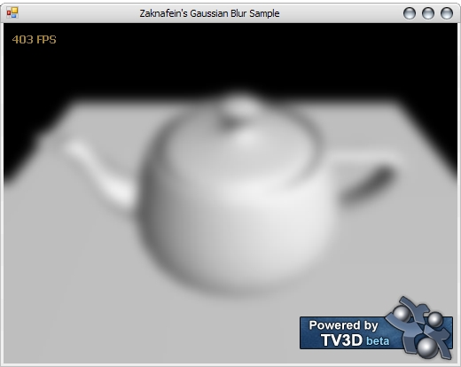
TV3D 6.5 Sample
Here it is! A VB.Net 2005 project showcasing an optimized gaussian blur shader, with a downsampling shader. It’s not for beginners, because there is strictly no comment, just well-written code. :)
Note : The demo does not yet reflect the updated formulas. It will come shortly.
GaussianBlur.rar [48kb]
Bonus (blurred) teapot!
Reference documents
As an alternative to the demo (which contains a GaussianDistribution class that does everything that the Excel file does), I have made a nice reference sheet on the 1D and 2D gaussian distribution functions, well I happen to have made one in Excel and a PDF version for those without MS Office. The Excel version is dynamic, so changing the σ will update all the functions.
Update : Cleaned and updated to reflect my newest findings! (augmentation and standard deviation calculation)
Enjoy!
Awsome, thanks for sharing Zak! I’m working on HDR and blurring is one of the areas I’m investing a fair amount of time into, in order to speed things up. =)
That would be much appreciated, thank you =) I copied the nvidia blurring sample (post gloom or something like that), and I’m sure it’s a little less than optimized.
Nice info and useful excel document, thanks! :) I will link this article from my page.
Since you normalize the weights for the blur you can remove the 1/sqrt(2*pi*thea). This a normalization factor and your blend weights will come out the same.
Very informative! I just learned here: http://www.coreldraw.com/en/pages/gaussian-blur/index.html about blur effect and how to add it but I need a lot of practice and as much informative stuff like this. Thank you for sharing it is very helpful