box filter – The Instruction Limit

First part can be found here.
An implementation of the concepts presented in this series can be found here.

The Perfect Sigma

The last post’s closing note was, how are we to find the “perfect” standard deviation for a fixed number of taps such that exactly 0% of light is lost. This means that the sum of all taps is exactly equal to 1.

It’s absolutely possible, but to find this exact σ with algebra and possibly calculus was a bit over my head. So I just “binary-searched” across the decimals until my Excel grid told me that as long as double-precision goes (15 significant numbers), I have ≈ 1 as the sum. I ended up with the following numbers :

17-tap : 1.2086
15-tap : 1.1402108
13-tap : 1.067359295
11-tap : 0.9890249035
9-tap : 0.90372907227
7-tap : 0.809171316279
5-tap : 0.7013915463849

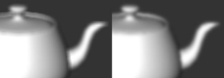
17-taps per pass, so basically 289 effective texture samples (actually 34…), and a standard deviation of 1.2?! This is what it looks like, original on right, blurred on left :

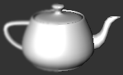
So my first thought was, “This can’t be right.”

Good Enough

In my first demo, I used a σ = 2.7 for 9 taps, and it didn’t look that bad.
So this got me thinking, how “boxy” can the Gaussian become for it to still look believable? Or, differently put, how much light can we lose before getting a Box-like filter?

To determine that, I needed a metric, a scale. I decided to use the Mean Difference, a.k.a. Average Deviation.
A Box filter does not vary, it’s constant, so its mean difference is always 0. By calculating how low my Gaussian approximations’ mean difference goes, one can find how similar it really is to a Box filter.

The upper limit (0% box-filter-similarity) would be the mean difference of a filter that loses no light at all, and the lower limit (100% similarity) would be equal to a box filter at (again) 15 significant decimal numbers.

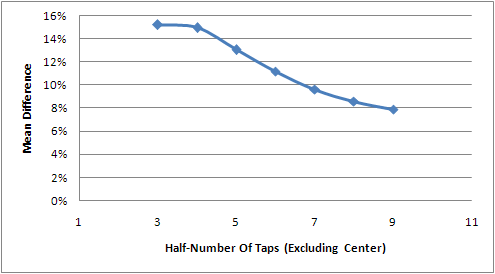
So I fired up Excel and made those calculations. It turns out that at 0% lost light, the mean difference is not linear with the number of taps. In fact, the shape highly resembles a bell curve :

I fitted this curve to a 4th order polynomial (which seemed to fit best in the graph) and at most, I got a 0.74% similarity for 0% lost light, in a 9-tap filter. I’m not looking for something perfect since this metric will be used for visual comparison; the whole process is highly subjective.

Eye Exam

Time to test an implementation and determine how much similarity is too much to this blogger’s eye.
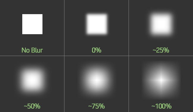
Here’s a fairly tiny 17×17 white square on a dark grey background, blurred with a 17-tap filter of varying σ and blown up 4 times with nearest-neighbour interpolation :

The percentage is my “box-likeness” or “box filter similarity” calculation described in the last section.

Up to 50%, I’m quite pleased with the results. The blurred halo feels very round and neat, with no box limit that cuts off the values harshly. But at 75%, it starts to look seriously boxy. In fact, anything bigger than 60% visibly cuts the blur off. And at 100%, it definitely doesn’t look like a Gaussian, more like a star with a boxy, diamond-shaped blur.

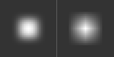
Here’s how 60% and 100% respectively look at a 9-tap, for comparison :

50% looks a liiiiiitle bit rounder, but 60% is still very acceptable and provide a nice blurring capability boost.

Conclusion

My conclusion, like my analysis, is extremely subjective…
I recommend not using more than 60% box-similarity (as calculated with my approach) to keep a good-looking Gaussian blur, and not more than 50% if your scene has very sharp contrasts/angles and you want optimal image quality.

The ideal case of 0% lost light is numerically perfect, but really unpractical in the real world. It feels like a waste of GPU cycles, and I don’t see any reason to limit ourselves to such low σ values.

Here’s a list of 50% and 60% standard deviations for all the tap counts that I consider practical for real-time shaders :

17-tap : 3.66 – 4.95
15-tap : 2.85 – 3.34
13-tap : 2.49 – 2.95
11-tap : 2.18 – 2.54
9-tap : 1.8 – 2.12
7-tap : 1.55 – 1.78
5-tap : 1.35 – 1.54

And last but not least, the Excel document (made with 2007 but saved as 2003 format) that I used to make this article : Gaussian Blur.xls

I hope you’ll find this useful! Me, I think I’m done with the Gaussian. :D

Second part can be found here.
An implementation of the concepts presented in this series can be found here.

A long time ago, in a blog not so far away, I studied how the Gaussian distribution worked to implement a Gaussian Blur HLSL shader. That worked pretty well, I learned a lot of stuff, and managed to make a very functional shader. But some problems were overlooked and fixed with not-so-scientific solutions/hacks. Last week and this week, I spent more time thinking and experimenting with Gaussian blur weights, and discovered some pretty interesting stuff.

Losing Light

The first problem that I mention in my original post is the fact that when passing any image through a Gaussian blur shader darkens it, a certain portion of brightness or “light” is lost in the process.
Usually, the Gaussian function (a.k.a. the bell curve or normal distribution) has an integral between from x = -∞ to +∞ of exactly 1. But when you sample it at discrete intervals, you always lose a certain portion of that full integral.
To prevent this effect, I decided to “normalize” all the weights (a weight being a sample of the G(x) function at some x distance) to have a sum of exactly one, since that’s what I want to end up with anyway. This works, and my filtered images are bright again.
But doing so has a subtle yet perverse effect to it.

Boxing the Gaussian

Let’s take a 5-tap uni-dimensional kernel with a standard deviation of σ = 1. As a reminder, the standard deviation defines how wide the function is, and how much blurring is performed, and the “tap” count is the number of texture samples done in a single pass (each pass being either horizontal or vertical).
Here are the weights acquired from the function, then the normalized weights (since the function is reflective at x = 0, I only show values for [0, 2]) :

0.39894228, 0.241970725, 0.053990967
Σ = 0.990865662
0.402619947, 0.244201342, 0.054488685
Σ = 1

That looks quite fine. Now let’s use a wider σ of 5.

0.079788456, 0.078208539, 0.073654028
Σ = 0.38351359
0.208045968, 0.203926382, 0.192050634
Σ = 1

Notice how the normalized weights are very close to each other. In fact, it highly resembles an averaging 5-tap Box filter :

0.2, 0.2, 0.2
Σ = 1

When you think about it’s it very natural for this effect to occur. The bigger the standard deviation, the closer to the curve’s apex you sample values, and the lower the apex as well. So the difference between the samples is smaller and you go closer to a straight line.
In fact, at σ = ∞, any normalized Gaussian kernel becomes a Box filter. I don’t have a formal proof for that, but it’s clearly visible, and with single-precision floats it takes a lot less than the infinity.

Visual Difference

Now why is it so bad to use a box filter? It’s as wide as our kernel can get with its limited number of taps after all…

Here’s a visual comparison of the same scene under a 5-tap Box filter and a Gaussian with σ ≈ 1.5, giving it about the same span. It’s not an apples-to-apples comparison, but it should give you an idea.

A Box filter is quite unlike a Gaussian blur. Sharp edges get blocky and it gives a more “sharp” feel than the Gaussian. So it’s definitely not optimal.

Ye Olde Cliffhanger

Getting late here, so I’ll wrap this up.
The question left is this one : At which standard deviation does our Gaussian sampling lose 0% brightness/light for a fixed number of taps? Is that even possible?
Why, yes, yes it is. I’ll keep this for part two!

Tag: box filter

Gaussian Blur Revisited, part two