Gaussian Blur Revisited, part one

Second part can be found here.
An implementation of the concepts presented in this series can be found here.

A long time ago, in a blog not so far away, I studied how the Gaussian distribution worked to implement a Gaussian Blur HLSL shader. That worked pretty well, I learned a lot of stuff, and managed to make a very functional shader. But some problems were overlooked and fixed with not-so-scientific solutions/hacks. Last week and this week, I spent more time thinking and experimenting with Gaussian blur weights, and discovered some pretty interesting stuff.

Losing Light

The first problem that I mention in my original post is the fact that when passing any image through a Gaussian blur shader darkens it, a certain portion of brightness or “light” is lost in the process.
Usually, the Gaussian function (a.k.a. the bell curve or normal distribution) has an integral between from x = -∞ to +∞ of exactly 1. But when you sample it at discrete intervals, you always lose a certain portion of that full integral.
To prevent this effect, I decided to “normalize” all the weights (a weight being a sample of the G(x) function at some x distance) to have a sum of exactly one, since that’s what I want to end up with anyway. This works, and my filtered images are bright again.
But doing so has a subtle yet perverse effect to it.

Boxing the Gaussian

Let’s take a 5-tap uni-dimensional kernel with a standard deviation of σ = 1. As a reminder, the standard deviation defines how wide the function is, and how much blurring is performed, and the “tap” count is the number of texture samples done in a single pass (each pass being either horizontal or vertical).
Here are the weights acquired from the function, then the normalized weights (since the function is reflective at x = 0, I only show values for [0, 2]) :

0.39894228, 0.241970725, 0.053990967
Σ = 0.990865662

0.402619947, 0.244201342, 0.054488685
Σ = 1

That looks quite fine. Now let’s use a wider σ of 5.

0.079788456, 0.078208539, 0.073654028
Σ = 0.38351359

0.208045968, 0.203926382, 0.192050634
Σ = 1

Notice how the normalized weights are very close to each other. In fact, it highly resembles an averaging 5-tap Box filter :

0.2, 0.2, 0.2
Σ = 1

When you think about it’s it very natural for this effect to occur. The bigger the standard deviation, the closer to the curve’s apex you sample values, and the lower the apex as well. So the difference between the samples is smaller and you go closer to a straight line.
In fact, at σ = ∞, any normalized Gaussian kernel becomes a Box filter. I don’t have a formal proof for that, but it’s clearly visible, and with single-precision floats it takes a lot less than the infinity.

Visual Difference

Now why is it so bad to use a box filter? It’s as wide as our kernel can get with its limited number of taps after all…

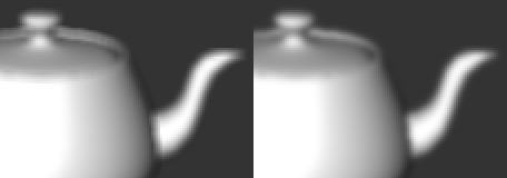
Here’s a visual comparison of the same scene under a 5-tap Box filter and a Gaussian with σ ≈ 1.5, giving it about the same span. It’s not an apples-to-apples comparison, but it should give you an idea.

A Box filter is quite unlike a Gaussian blur. Sharp edges get blocky and it gives a more “sharp” feel than the Gaussian. So it’s definitely not optimal.

Ye Olde Cliffhanger

Getting late here, so I’ll wrap this up.
The question left is this one : At which standard deviation does our Gaussian sampling lose 0% brightness/light for a fixed number of taps? Is that even possible?
Why, yes, yes it is. I’ll keep this for part two!